NISAR Access and Exploration
Authors: Harshini Girish (UAH), Rajat Shinde (UAH), Alex Mandel (Development Seed), Henry Rodman (Development Seed), Samantha Niemoeller (JPL)
Date: March 17, 2026
Description: In this tutorial, we discover a NISAR L2 GCOV Beta sample granule with earthaccess and then choose one of two access paths: direct S3 for users running inside NASA MAAP / AWS us-west-2, or authenticated HTTPS for users running outside that environment. After choosing one path, both workflows assign the selected file handle to a shared variable so the same exploration and visualization cells work without manual renaming.
Run This Notebook
To access and run this tutorial within MAAP’s Algorithm Development Environment (ADE), please refer to the “Getting started with the MAAP” section of our documentation.
This notebook supports two separate access workflows:
S3 workflow: use this when you are running inside NASA MAAP / AWS us-west-2.
HTTPS workflow: use this when you are running outside that environment, including ESA MAAP or a local machine with valid Earthdata Login credentials.
Run the import and discovery cells first, then run only one of the two access paths. Once you reach the Choose the file object for the rest of the notebook cell, the later exploration and visualization cells are shared.
About the Data
This tutorial uses NISAR Sample L-band products hosted by ASF/NASA Earthdata. These are sample datasets intended to help users practice discovery and access patterns before routine NISAR science products are broadly available. For this workflow, we focus on the Level-2 Geocoded Polarimetric Covariance (GCOV) sample product. GCOV provides geocoded covariance information (for the available polarization channels) on a map grid, making it well-suited for quick inspection and visualization in Python. Although these are sample files (not full global-scale operational coverage), they are designed to be structurally compatible with the expected NISAR product format, so the same access and exploration steps can be reused for future NISAR GCOV data.
Data reference: NISAR Sample L-band GCOV granules (Earthdata Search)
Additional Resources
Import and Install Packages
[ ]:
from maap.maap import MAAP
import xarray as xr
import s3fs
import earthaccess
import rioxarray
import matplotlib.pyplot as plt
import os
import h5py
import numpy as np
from rasterio.transform import from_origin
maap = MAAP()
Access the Data
In this section we show two practical access patterns for GCOV files:
Direct S3 using temporary AWS credentials. This is the recommended workflow when running inside NASA MAAP / AWS us-west-2.
HTTPS using Earthdata Login authentication. This is the recommended workflow when running outside that environment.
After you open the file using one of these methods, both workflows feed into the same shared variable, nisar_file_obj, so the later exploration and visualization cells do not need to be edited.
Querying Method 1: via the maap-py
The first method uses maap-py to request temporary AWS credentials(via ASF) and configure s3fs for direct S3 access. This is the recommended cloud-first workflow when running in the MAAP environment (ADE/DPS) because it enables streaming reads from the s3://... asset without downloading the full file.
[2]:
asf_s3 = "https://nisar.asf.earthdatacloud.nasa.gov/s3credentials"
creds = maap.aws.earthdata_s3_credentials(asf_s3)

fs_s3 = s3fs.S3FileSystem(
    anon=False,
    key=creds["accessKeyId"],
    secret=creds["secretAccessKey"],
    token=creds["sessionToken"],
)
Querying Method 2: via earthaccess
earthaccess works inside and outside the MAAP ADE/DPS. Use it for a portable Earthdata Login (EDL) workflow—especially when opening GCOV via the HTTPS asset link. If .netrc or environment variables are not set, it will prompt for your EDL credentials (input hidden).
For more information, see Authentication: Before we can use earthaccess we need an account with NASA EDL.
[3]:
earthaccess.login()

results = earthaccess.search_data(
    short_name="NISAR_L2_GCOV_BETA_V1",
    count=10,
    cloud_hosted=True,
)

print("Granules found:", len(results))
g = results[0]
Granules found: 10
Get access links (HTTPS + direct S3)
We resolve the chosen granule into both HTTPS and direct S3 links. You do not need to use both.
Use ``s3_link`` for the S3 workflow inside NASA MAAP / AWS us-west-2.
Use ``https_link`` for the HTTPS workflow outside that environment.
[4]:
https_link = g.data_links()[0]
s3_link = g.data_links(access="direct")[0]
Open the Cloud-Optimized HDF5
The next few cells prepare runtime read settings and then show the two separate access paths. Run the setup cell and then run only the path that matches your environment.
Setup parameters for cloud-optimized access
When streaming large HDF5/NetCDF-style files from cloud object storage, performance is dominated by how many small random reads you trigger. We (1) enable fsspec block caching (cache_type="blockcache") so reads are grouped into MB-sized blocks (block_size=8MB), and (2) tune HDF5 runtime caches via h5py driver keywords (page_buf_size=16MB, rdcc_nbytes=4MB) to reduce metadata/data thrashing during chunked access. These settings are runtime read parameters (not
intrinsic file properties), and if you omit them the file can still open remotely but may be noticeably slower/less stable for large HDF5 datasets. For GCOV, these defaults have worked consistently so far and are safe to copy-paste; adjust if future specs recommend different values.
See the “Cloud-Optimized NetCDF4/HDF5 Guide” for more details
[5]:
# Cloud-optimized I/O tuning
io_params = {
    "fsspec_params": {
        "cache_type": "blockcache",
        "block_size": 8 * 1024 * 1024,   # 8MB blocks
    },
    "h5py_params": {
        "driver_kwds": {
            "page_buf_size": 16 * 1024 * 1024,  # 16MB page buffer
            "rdcc_nbytes": 4 * 1024 * 1024,     # 4MB chunk cache
        }
    }
}

#output
print("File:", https_link.split("/")[-1])
print("HTTPS:", https_link)
print("S3:", s3_link)
File: NISAR_L2_PR_GCOV_002_109_D_063_4005_DHDH_A_20251012T182508_20251012T182531_X05010_N_P_J_001.h5
HTTPS: https://nisar.asf.earthdatacloud.nasa.gov/NISAR/NISAR_L2_GCOV_BETA_V1/NISAR_L2_PR_GCOV_002_109_D_063_4005_DHDH_A_20251012T182508_20251012T182531_X05010_N_P_J_001/NISAR_L2_PR_GCOV_002_109_D_063_4005_DHDH_A_20251012T182508_20251012T182531_X05010_N_P_J_001.h5
S3: s3://sds-n-cumulus-prod-nisar-products/NISAR_L2_GCOV_BETA_V1/NISAR_L2_PR_GCOV_002_109_D_063_4005_DHDH_A_20251012T182508_20251012T182531_X05010_N_P_J_001/NISAR_L2_PR_GCOV_002_109_D_063_4005_DHDH_A_20251012T182508_20251012T182531_X05010_N_P_J_001.h5
Path A: Open via direct S3 link
Use this path when you are running inside NASA MAAP / AWS us-west-2 and have temporary AWS credentials available. This keeps the workflow cloud-first by streaming only what is needed from the HDF5 file instead of downloading the full granule.
[6]:
# Open the NISAR HDF5 over S3
nisar_file_obj_s3 = fs_s3.open(s3_link, mode="rb", **io_params["fsspec_params"])
nisar_file_obj_s3
[6]:
<File-like object S3FileSystem, sds-n-cumulus-prod-nisar-products/NISAR_L2_GCOV_BETA_V1/NISAR_L2_PR_GCOV_002_109_D_063_4005_DHDH_A_20251012T182508_20251012T182531_X05010_N_P_J_001/NISAR_L2_PR_GCOV_002_109_D_063_4005_DHDH_A_20251012T182508_20251012T182531_X05010_N_P_J_001.h5>
Path B: Open via HTTPS link
Use this path when you are running outside NASA MAAP / AWS us-west-2. This opens the HTTPS asset as a file-like object using an authenticated fsspec session, again without downloading the full file.
[7]:
fs_https = earthaccess.get_fsspec_https_session()
nisar_file_obj_https = fs_https.open(https_link, mode="rb", **io_params["fsspec_params"])
nisar_file_obj_https
[7]:
<File-like object HTTPFileSystem, https://nisar.asf.earthdatacloud.nasa.gov/NISAR/NISAR_L2_GCOV_BETA_V1/NISAR_L2_PR_GCOV_002_109_D_063_4005_DHDH_A_20251012T182508_20251012T182531_X05010_N_P_J_001/NISAR_L2_PR_GCOV_002_109_D_063_4005_DHDH_A_20251012T182508_20251012T182531_X05010_N_P_J_001.h5>
Choose the file object for the rest of the notebook
Run one of the two open-file paths above, then use the matching assignment below. Keep only the line that matches the workflow you ran.
[8]:
# Choose one of the following based on the path you ran above:

# For Path A (direct S3 inside NASA MAAP / AWS us-west-2):
nisar_file_obj = nisar_file_obj_s3

# For Path B (HTTPS outside NASA MAAP / AWS us-west-2):
# nisar_file_obj = nisar_file_obj_https
The remaining cells below use nisar_file_obj. Once you assign that shared variable, you should not need to rename _s3 or _https anywhere else in the notebook.
Explore the Data
The GCOV HDF5s contain rich metadata and multiple grids. To keep the tutorial readable we inspect a focused subset of the tree—specifically the primary grid group used for plotting: GCOV/grids/frequencyA.
Open the selected file for exploration
After assigning nisar_file_obj above, run the next cell to open the selected GCOV file as an xarray DataTree.
[ ]:
dt = xr.open_datatree(
    nisar_file_obj,
    engine="h5netcdf",
    phony_dims="sort",
    **io_params["h5py_params"]
)
[10]:
dt["science"]["LSAR"]["GCOV"]["grids"]["frequencyA"].keys()
[10]:
KeysView(<xarray.DataTree 'frequencyA'>
Group: /science/LSAR/GCOV/grids/frequencyA
    Dimensions:                (yCoordinates: 36720, xCoordinates: 37080,
                                phony_dim_2: 2)
    Coordinates:
      * yCoordinates           (yCoordinates) float64 294kB 5.76e+06 ... 5.393e+06
      * xCoordinates           (xCoordinates) float64 297kB 1.483e+05 ... 5.191e+05
    Dimensions without coordinates: phony_dim_2
    Data variables:
        HHHH                   (yCoordinates, xCoordinates) float32 5GB ...
        HVHV                   (yCoordinates, xCoordinates) float32 5GB ...
        listOfCovarianceTerms  (phony_dim_2) |S4 8B ...
        listOfPolarizations    (phony_dim_2) |S2 4B ...
        mask                   (yCoordinates, xCoordinates) float32 5GB ...
        numberOfLooks          (yCoordinates, xCoordinates) float32 5GB ...
        numberOfSubSwaths      uint8 1B ...
        projection             uint32 4B ...
        rtcGammaToSigmaFactor  (yCoordinates, xCoordinates) float32 5GB ...
        xCoordinateSpacing     float64 8B ...
        yCoordinateSpacing     float64 8B ...)
Visualize the Data
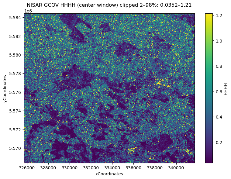
This cell plots the NISAR L2 GCOV HHHH layer using the shared file object selected above. It opens only the /science/LSAR/GCOV/grids/frequencyA group (no full download and no Dask), uses engine="h5netcdf" with phony_dims="sort", and drops listOfCovarianceTerms / listOfPolarizations to avoid dimension-related read issues. After loading a small center window, it computes robust color limits using the 2nd–98th percentiles and renders the window with pcolormesh using the
native xCoordinates and yCoordinates axes.
[11]:
gcov_group = "/science/LSAR/GCOV/grids/frequencyA"

ds_gcov = xr.open_dataset(
    nisar_file_obj,
    engine="h5netcdf",
    group=gcov_group,
    phony_dims="sort",
    drop_variables=["listOfCovarianceTerms", "listOfPolarizations"],
    **io_params["h5py_params"]
)

da = ds_gcov["HHHH"]
y = ds_gcov["yCoordinates"]
x = ds_gcov["xCoordinates"]

half = 800
ny, nx = da.sizes["yCoordinates"], da.sizes["xCoordinates"]
cy, cx = ny // 2, nx // 2
y0, y1 = max(0, cy - half), min(ny, cy + half)
x0, x1 = max(0, cx - half), min(nx, cx + half)

da_win = da.isel(yCoordinates=slice(y0, y1), xCoordinates=slice(x0, x1)).load()
x_win = x.isel(xCoordinates=slice(x0, x1)).load()
y_win = y.isel(yCoordinates=slice(y0, y1)).load()

arr = np.asarray(da_win.values).astype("float32")
vmin = float(np.percentile(arr, 2))
vmax = float(np.percentile(arr, 98))

plt.figure(figsize=(8, 6))
plt.pcolormesh(x_win, y_win, arr, shading="auto", vmin=vmin, vmax=vmax)
plt.title(f"NISAR GCOV HHHH (center window) clipped 2–98%: {vmin:.3g}–{vmax:.3g}")
plt.xlabel("xCoordinates")
plt.ylabel("yCoordinates")
plt.colorbar(label="HHHH")
plt.tight_layout()
plt.show()