Accessing EDAV Data via Web Coverage Service
Authors: Alex Mandel (Development Seed), Samuel Ayers (UAH), Aimee Barciauskas (Development Seed)
Date: April 3, 2023
Description: This example demonstrates how to retrieve raster data from EDAV using a Web Coverage Service (WCS). A WCS lets you access coverage data with multiple dimensions online. The downloaded data is subsetted from data hosted on the MAAP and is available with the full resolution and values.
Run This Notebook
To access and run this tutorial within MAAP’s Algorithm Development Environment (ADE), please refer to the “Getting started with the MAAP” section of our documentation.
Disclaimer: it is recommended to run this tutorial within MAAP’s ADE Pangeo workspace, which already includes rioxarray.
Additional Resources
Importing and Installing Packages
We start by installing the libraries that are used to query the WCS connection point, and then to load, explore, and plot the raster data. We use rasterio for reading and writing raster formats, rio-cogeo for creating and validating Cloud Optimized GEOTIFF (COG) data, and owslib for interacting with Open Geospatial Consortium (OGC) services.
[ ]:
# install libraries
# %pip is a magic command that installs into the current kernel
# -q means quiet (to give less output)
%pip install -q rasterio
%pip install -q rio-cogeo
%pip install -q owslib
After installing the libraries, note that you may see multiple messages that you need to restart the kernel. Then import rasterio, show from rasterio.plot to display images with labeled axes, and WebCoverageService from owslib.wcs to program with an OGC web service.
[46]:
# import rasterio
import rasterio as rio
# import show
from rasterio.plot import show
# import WebCoverageService
from owslib.wcs import WebCoverageService
Querying the WCS
Now we can configure the WCS source, use the getCoverage function to request a file in GeoTIFF format, and save what is returned to our workspace.
[47]:
# configure the WCS source
EDAV_WCS_Base = "https://edav-das.val.esa-maap.org/wcs"
wcs = WebCoverageService(f'{EDAV_WCS_Base}?service=WCS', version='2.0.0')
[48]:
# request imagery to download
response = wcs.getCoverage(
    identifier=['ESACCI_Biomass_L4_AGB'], # coverage ID
    format='image/tiff', # format what the coverage response will be returned as
    filter='false', # define constraints on query
    scale=1, # resampling factor (1 full resolution, 0.1 resolution degraded of a factor of 10)
    subsets=[('Long',11.54,11.8),('Lat',-0.3,0.0)] # subset the image by lat / lon
)

# save the results to file as a tiff
results = "EDAV_example.tif"
with open(results, 'wb') as file:
    file.write(response.read())
We can use gdalinfo to provide information about our raster dataset to make sure the data is valid and contains spatial metadata.
[49]:
# gives information about the dataset
!gdalinfo {results}
Driver: GTiff/GeoTIFF
Files: EDAV_example.tif
Size is 293, 339
Warning 1: PROJ: proj_create_from_database: Open of /opt/conda/share/proj failed
Coordinate System is:
GEOGCRS["WGS 84",
    DATUM["World Geodetic System 1984",
        ELLIPSOID["WGS 84",6378137,298.257223563,
            LENGTHUNIT["metre",1,
                ID["EPSG",9001]]]],
    PRIMEM["Greenwich",0,
        ANGLEUNIT["degree",0.0174532925199433,
            ID["EPSG",9122]]],
    CS[ellipsoidal,2],
        AXIS["latitude",north,
            ORDER[1],
            ANGLEUNIT["degree",0.0174532925199433,
                ID["EPSG",9122]]],
        AXIS["longitude",east,
            ORDER[2],
            ANGLEUNIT["degree",0.0174532925199433,
                ID["EPSG",9122]]]]
Data axis to CRS axis mapping: 2,1
Origin = (11.539555555748001,0.000888887639000)
Pixel Size = (0.000888888889000,-0.000888888889000)
Metadata:
  AREA_OR_POINT=Area
  cdm_data_type=INT
  comment=These data were produced at ESA CCI as part of the ESA Biomass CCI project.
  Conventions=CF-1.7
  creator_email=santoro@gamma-rs.ch
  creator_name=GAMMA Remote Sensing
  creator_url=www.gamma-rs.ch
  date_created=2021-6-3
  EPSG=4326
  format_version=CCI Data Standards v2.1
  geospatial_lat_max=0
  geospatial_lat_min=-10
  geospatial_lat_resolution=0.00088889
  geospatial_lat_units=degrees_north
  geospatial_lon_max=20
  geospatial_lon_min=10
  geospatial_lon_resolution=0.00088889
  geospatial_lon_units=degrees_east
  geospatial_vertical_max=0.0
  geospatial_vertical_min=0.0
  history=AGB estimation with BIOMASAR-L, v202101, AGB estimation with BIOMASAR-C, v202101, Merging of AGB estimates, v202101
  id=N00E010_ESACCI-BIOMASS-L4-AGB_SD-MERGED-100m-${year}-fv3.0.tif
  institution=GAMMA Remote Sensing
  keywords=satellite, observation, forest, biomass
  keywords_vocabulary=NASA Global Change Master Directory (GCMD) Science Keywords
  key_variables=AGB
  license=ESA CCI Data Policy: free and open access
  naming authority=ch.gamma-rs
  platform=ALOS-1 PALSAR, ENVISAT ASAR
  product_version=3.0
  proj4=+proj=longlat +datum=WGS84 +no_defs
  project=Climate Change Initiative - European Space Agency
  references=http://cci.esa.int/biomass
  sensor=PALSAR, SAR-C
  source=ALOS-1 PALSAR FB mosaics, ENVISAT ASAR WideSwath
  spatial_resolution=100 m
  standard_name_vocabulary=NetCDF Climate and Forecast (CF) Metadata Convention version 67
  summary=This dataset contains a global map of above-ground biomass of the epoch 2010 obtained from L-and C-band spaceborne SAR backscatter, placed onto a regular grid.
  time_coverage_duration=P1Y
  time_coverage_end=20101231T235959Z
  time_coverage_resolution=P1Y
  time_coverage_start=20100101T000000Z
  title=ESA CCI above-ground biomass standard deviation product level 4, year 2010
  tracking_id=30d2a523-05a8-44ce-8c19-a37b5feb2cf7
Image Structure Metadata:
  COMPRESSION=LZW
  INTERLEAVE=BAND
Corner Coordinates:
Upper Left  (  11.5395556,   0.0008889) ( 11d32'22.40"E,  0d 0' 3.20"N)
Lower Left  (  11.5395556,  -0.3004444) ( 11d32'22.40"E,  0d18' 1.60"S)
Upper Right (  11.8000000,   0.0008889) ( 11d48' 0.00"E,  0d 0' 3.20"N)
Lower Right (  11.8000000,  -0.3004444) ( 11d48' 0.00"E,  0d18' 1.60"S)
Center      (  11.6697778,  -0.1497778) ( 11d40'11.20"E,  0d 8'59.20"S)
Band 1 Block=293x13 Type=UInt16, ColorInterp=Gray
  NoData Value=0
Reading the Data
We can now use rio.open with our results path string and return an opened dataset object. We can set a variable (rast) to what is read from this dataset object. Then, we utilize the function show to display the raster using Matplotlib.
[50]:
# take path and return opened dataset object, set variable to read dataset object
with rio.open(results, 'r') as src:
        rast = src.read()
[51]:
# make a plot
show(rast, transform=src.transform, cmap='pink')
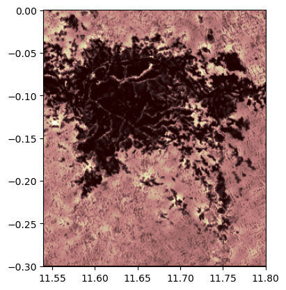
[51]:
<AxesSubplot: >
We now have a visual of our raster. Let’s import and employ the show_hist function from rasterio.plot to generate a histogram of the raster.
[52]:
# import show_hist
from rasterio.plot import show_hist
# create histogram
show_hist(rast,
          bins=50,# number of bins to compute histogram across
          alpha=.3,# transparency
          title="Histogram"# figure title
         )
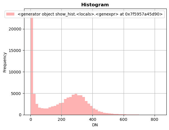
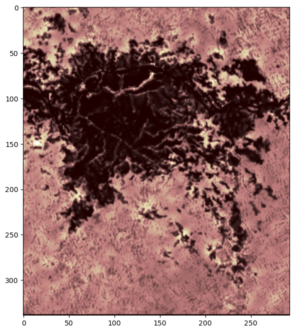
We can also generate a plot using Matplotlib. Let’s import matplotlib.pyplot and numpy and make a new plot. To do this, use the plt.subplots function to return a figure and a single “Axes” instance. Then remove single-dimensional entries from the shape of our array using np.squeeze and display the data as an image using imshow. Now, we can set the norm limits for image scaling using the set_clim function.
[53]:
# import matplotlib.pyplot
import matplotlib.pyplot as plt
# import numpy
import numpy as np
[54]:
# set figure and single "Axes" instance
fig, ax = plt.subplots(1, figsize=(8,8))
# remove single-dimensional entries from the shape of the variable rast
#     and display the image
edavplot = ax.imshow(np.squeeze(rast), cmap='pink')
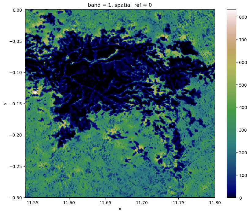
Newer Method rioxarray
Another way to work with raster data is with the rasterio “xarray” extension. Let’s install and import rioxarray and create a plot using the open_rasterio and plot functions.
[ ]:
# install rasterio xarray extension
%pip install -q rioxarray
[56]:
# import rasterio xarray extension
import rioxarray
[57]:
# opens results with rasterio to set dataarray
edav_x = rioxarray.open_rasterio(results)
[58]:
# plot dataarray
edav_x.plot(cmap="gist_earth", figsize=(10,8))
[58]:
<matplotlib.collections.QuadMesh at 0x7f591617ae60>