NISAR DEM (v1.2): Access and Visualize

Date: March 4, 2026

Author: Harshini Girish (UAH), Rajat Shinde (UAH), Alex Mandel (Development Seed), Jamison French (Development Seed), Brian Freitag (NASA MSFC), Sheyenne Kirkland (UAH), Henry Rodman (Development Seed), Zac Deziel (Development Seed), Chuck Daniels (Development Seed)

Description: This notebook subsets a small Area of Interest (AOI) from the NISAR DEM VRT stored in ASF’s S3 bucket using rasterio’s AWSSession together with rasterio.Env for authenticated requester-pays S3 access. It logs in via Earthdata, requests temporary S3 credentials, opens the DEM directly from S3, clips the AOI in memory with rioxarray, and plots the result for quick inspection. This example intentionally focuses on access and in-memory subsetting; for a related MAAP example that writes an Xarray object to a cloud-optimized GeoTIFF (COG), see the Additional Resources section below.

Run This Notebook

To access and run this tutorial within MAAP’s Algorithm Development Environment (ADE), please refer to the “Getting started with the MAAP” section of our documentation.

Disclaimer: it is highly recommended to run a tutorial within MAAP’s ADE, which already includes packages specific to MAAP, such as maap-py. Running the tutorial outside of the MAAP ADE may lead to errors. Additionally, it is recommended to use the Pangeo workspace within the ADE, since certain packages relevant to this tutorial are already installed.

About the Data

This notebook uses the NISAR DEM v1.2 collection hosted by the NASA Alaska Satellite Facility (ASF) DAAC. It is a global digital elevation model (DEM) prepared for NISAR processing workflows and is not derived from NISAR measurements; instead, it is modified from the Copernicus DEM 30 m source product. Key modifications include converting the vertical reference from the EGM2008 geoid to the WGS84 ellipsoid, filling gaps (e.g., over ocean / missing tiles) to provide complete global coverage, and publishing the data through a hierarchical VRT (Virtual Raster) structure for fast, unified access. The top-level VRT file (``EPSG4326.vrt``) points to a second tier of VRTs organized by latitude bands, which in turn reference the underlying tiles; this makes it easy to access the DEM as one “virtual mosaic” without manually managing tile lists. Note: because elevations are ellipsoid-referenced, this dataset should not be used for applications that specifically require geoid-based elevations.

Additional Resources

• NISAR Access

• Searching NISAR + BIOMASS Overlapping Data

• ESA CCI Biomass V5.01 — Saving Tile as COG

For a related MAAP science example that shows writing a cloud-optimized GeoTIFF (COG) from an Xarray-backed workflow, see ESA CCI Biomass V5.01 — Saving Tile as COG above.

Imports

Load all required libraries (earthaccess for authentication, rasterio for S3 access/session handling, rioxarray for in-memory clipping, and matplotlib for previewing the subset).

import time

import matplotlib.pyplot as plt
import rasterio
import rioxarray
from rasterio.session import AWSSession

import earthaccess

Parameters

Define the DEM version/projection directory and the AOI bounding box to subset.

# --- DEM version + projection directory ---
DEM_VERSION = "v1.2"
EPSG_DIR = "EPSG4326"  # also available: "EPSG3413" (Arctic), "EPSG3031" (Antarctic)

# --- AOI bbox ---
# For EPSG4326: lon/lat bbox (min_lon, min_lat, max_lon, max_lat)
BBOX = (-116.7, 35.9, -116.6, 36.0)

VRT paths

Construct the VRT path in ASF’s S3 bucket. The /vsis3/ path is what rasterio/GDAL will read directly from S3.

# --- ASF S3 VRT (DEM mosaic as a VRT) ---
ASF_S3_BUCKET = "sds-n-cumulus-prod-nisar-products"
S3_KEY = f"DEM/{DEM_VERSION}/{EPSG_DIR}/{EPSG_DIR}.vrt"

S3_VRT_S3URI = f"s3://{ASF_S3_BUCKET}/{S3_KEY}"
S3_VRT_VSI = f"/vsis3/{ASF_S3_BUCKET}/{S3_KEY}"

S3_VRT_S3URI

's3://sds-n-cumulus-prod-nisar-products/DEM/v1.2/EPSG4326/EPSG4326.vrt'

Set up Access

Log in via Earthdata and request short-lived S3 credentials from ASF so the S3 VRT can be accessed.

#Fetch temporary S3 credentials via Earthdata login
ASF_S3CREDS_ENDPOINT = "https://nisar.asf.earthdatacloud.nasa.gov/s3credentials"

auth = earthaccess.login()

creds = None
for attempt in range(1, 6):
    try:
        creds = auth.get_s3_credentials(endpoint=ASF_S3CREDS_ENDPOINT)
        print(f"Got S3 creds on attempt {attempt}")
        break
    except Exception as e:
        print(f"Attempt {attempt} failed:", type(e).__name__, e)
        time.sleep(5)

if creds is None:
    raise RuntimeError("Could not obtain ASF S3 credentials after retries.")

Got S3 creds on attempt 1

AWS session setup

Create a rasterio AWSSession from the temporary ASF S3 credentials and use it with rasterio.Env for requester-pays S3 access.

session = AWSSession(
    aws_access_key_id=creds["accessKeyId"],
    aws_secret_access_key=creds["secretAccessKey"],
    aws_session_token=creds["sessionToken"],
    region_name="us-west-2",
    requester_pays=True,
)

Subsetting helper

Define a helper function that opens the DEM from S3 inside a rasterio environment and clips the AOI in memory with rioxarray.

def open_dem_subset(dataset_path: str, bbox, session: AWSSession):
    """Open a DEM from S3 and clip the requested bounding box in memory."""
    minx, miny, maxx, maxy = bbox

    with rasterio.Env(session=session):
        rds = rioxarray.open_rasterio(dataset_path, mask_and_scale=True)
        clipped = rds.rio.clip_box(minx=minx, miny=miny, maxx=maxx, maxy=maxy).load()

    return clipped

Run subset in memory

Open the S3 VRT with the AWS session and clip the AOI in memory.

try:
    clipped = open_dem_subset(S3_VRT_S3URI, BBOX, session)
    print("Subset loaded in memory")
    print("CRS:", clipped.rio.crs)
    print("Bounds:", clipped.rio.bounds())
except Exception as e:
    print("S3 subset failed:", type(e).__name__, e)
    raise

Subset loaded in memory
CRS: EPSG:4326
Bounds: (-116.70013888888889, 35.89986111111111, -116.59986111111111, 36.00013888888889)

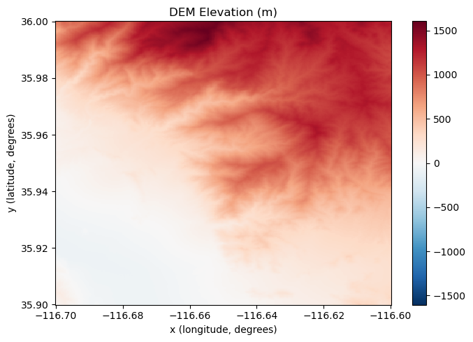
Preview

Plot the clipped DEM directly from the in-memory Xarray object.

plt.figure(figsize=(7, 5))
clipped.squeeze().plot.imshow()
plt.title("DEM Elevation (m)")
plt.xlabel(f"{clipped.squeeze().dims[-1]} (longitude, degrees)")
plt.ylabel(f"{clipped.squeeze().dims[-2]} (latitude, degrees)")
plt.tight_layout()
plt.show()